Introduction to algorithms
Algorithms
Algorithm is ‘a formally defined procedure for performing some calculation’. If a procedure is formally defined, then it can be implemented using a formal language, and such a language is known as a programming language. In general terms, an algorithm provides a blueprint to write a program to solve a particular problem. It is considered to be an effective procedure for solving a problem in finite number of steps. That is, a well-defined algorithm always provides an answer and is guaranteed to terminate.
Algorithms are mainly used to achieve software reuse. Once we have an idea or a blueprint of a solution, we can implement it in any high-level language like C, C++, or Java.
An algorithm is basically a set of instructions that solve a problem. It is not uncommon to have multiple algorithms to tackle the same problem, but the choice of a particular algorithm must depend on the time and space complexity of the algorithm.
DIFFERENT APPROACHES TO DESIGNING AN ALGORITHM
Algorithms are used to manipulate the data contained in data structures. When working with data structures, algorithms are used to perform operations on the stored data.
A complex algorithm is often divided into smaller units called modules. This process of dividing an algorithm into modules is called modularization. The key advantages of modularization are as follows:
It makes the complex algorithm simpler to design and implement.
Each module can be designed independently. While designing one module, the details of other modules can be ignored, thereby enhancing clarity in design which in turn simplifies implementation, debugging, testing, documenting, and maintenance of the overall algorithm.
There are two main approaches to design an algorithm—top-down approach and bottom-up approach, as shown in Figure below: -
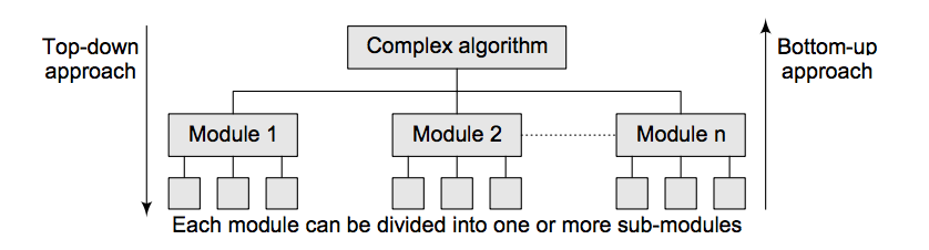
Fig. Different approaches of designing an algorithm
Top-down approach A top-down design approach starts by dividing the complex algorithm into one or more modules. These modules can further be decomposed into one or more sub-modules, and this process of decomposition is iterated until the desired level of module complexity is achieved. Top-down design method is a form of stepwise refinement where we begin with the topmost module and incrementally add modules that it calls.
Therefore, in a top-down approach, we start from an abstract design and then at each step, this design is refined into more concrete levels until a level is reached that requires no further refinement.
Bottom-up approach A bottom-up approach is just the reverse of top-down approach. In the bottom-up design, we start with designing the most basic or concrete modules and then proceed towards designing higher level modules. The higher level modules are implemented by using the operations performed by lower level modules. Thus, in this approach sub-modules are grouped together to form a higher level module. All the higher level modules are clubbed together to form even higher level modules. This process is repeated until the design of the complete algorithm is obtained.
CONTROL STRUCTURES USED IN ALGORITHMS
An algorithm has a finite number of steps. Some steps may involve decision-making and repetition. Broadly speaking, an algorithm may employ one of the following control structures: (a) sequence, (b) decision, and (c) repetition.
Sequence
By sequence, we mean that each step of an algorithm is executed in a specified order. Let us write an algorithm to add two numbers. This algorithm performs the steps in a purely sequential order, as shown below :-
Step 1 : Input first number as A

Step 2 : Input second number as B

Step 3 :  Set SUM = A+B

Step 4 : print SUM

Step 5 : END
Decision
Decision statements are used when the execution of a process depends on the outcome of some condition.
A decision statement can also be stated in the following manner:
IF condition

        Then process1

ELSE
        process2
Example:
Step 1 : Input first number as A

Step 2 : Input second number as B

Step 3 :  IF  A=B

                    Print “EQUAL”

              ELSE

                    Print “NOT EQUAL”

             [END of IF]

Step 5 : END
Repetition
Repetition, which involves executing one or more steps for a number of times, can be implemented using constructs such as while, do–while, and for loops. These loops execute one or more steps until some condition is true.
Step 1: [INITIALIZE] set I=1, N=10

Step 2: Repeat step 3 and 4 WHILE I<=N

Step 3: PRINT I, set I=I+1

            [END of LOOP]

Step 4: END
TIME AND SPACE COMPLEXITY
Analyzing an algorithm means determining the amount of resources (such as time and memory) needed to execute it. Algorithms are generally designed to work with an arbitrary number of inputs, so the efficiency or complexity of an algorithm is stated in terms of time and space complexity.
The time complexity of an algorithm is basically the running time of a program as a function of the input size. Similarly, the space complexity of an algorithm is the amount of computer memory that is required during the program execution as a function of the input size.
In other words, the number of machine instructions which a program executes is called its time complexity. This number is primarily dependent on the size of the program’s input and the algorithm used.
Generally, the space needed by a program depends on the following two parts:
Fixed part: It varies from problem to problem. It includes the space needed for storing instructions, constants, variables, and structured variables (like arrays and structures).
Variable part: It varies from program to program. It includes the space needed for recursion stack, and for structured variables that are allocated space dynamically during the runtime of a program.
However, running time requirements are more critical than memory requirements. Therefore, we will concentrate on the running time efficiency of algorithms.
Worst-Case, Best-Case, and Average-Case Efficiencies
We have established that it is reasonable to measure an algorithm’s efficiency as a function of a parameter indicating the size of the algorithm’s input. But there are many algorithms for which running time depends not only on an input size but also on the specifics of a particular input.
Consider, as an example, sequential search. This is a straightforward algorithm that searches for a given item (some search key K) in a list of n elements by checking successive elements of the list until either a match with the search key is found or the list is exhausted.
Here is the algorithm’s pseudocode, in which, for simplicity, a list is implemented as an array.
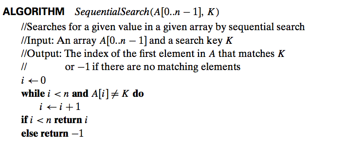
Clearly, the running time of this algorithm can be quite different for the same list size n. In the worst case, when there are no matching elements or the first matching element happens to be the last one on the list, the algorithm makes the largest number of key comparisons among all possible inputs of size n: Cworst(n) = n.
The worst-case efficiency of an algorithm is its efficiency for the worst-case input of size n, which is an input (or inputs) of size n for which the algorithm runs the longest among all possible inputs of that size. The way to determine the worst-case efficiency of an algorithm is, in principle, quite straightforward: analyze the algorithm to see what kind of inputs yield the largest value of the basic operation’s count C(n) among all possible inputs of size n and then compute this worst-case value Cworst(n).
The best-case efficiency of an algorithm is its efficiency for the best-case input of size n, which is an input (or inputs) of size n for which the algorithm runs the fastest among all possible inputs of that size. Accordingly, we can analyze the best- case efficiency as follows. First, we determine the kind of inputs for which the count C(n) will be the smallest among all possible inputs of size n. (Note that the best case does not mean the smallest input; it means the input of size n for which the algorithm runs the fastest.) Then we ascertain the value of C(n) on these most convenient inputs. For example, the best-case inputs for sequential search are lists of size n with their first element equal to a search key; accordingly, Cbest (n) = 1 for this algorithm.
The analysis of the best-case efficiency is not nearly as important as that of the worst-case efficiency. But it is not completely useless, either. Though we should not expect to get best-case inputs, we might be able to take advantage of the fact that for some algorithms a good best-case performance extends to some useful types of inputs close to being the best-case ones. For example, there is a sorting algorithm (insertion sort) for which the best-case inputs are already sorted arrays on which the algorithm works very fast. Moreover, the best-case efficiency deteriorates only slightly for almost-sorted arrays. Therefore, such an algorithm might well be the method of choice for applications dealing with almost-sorted arrays. And, of course, if the best-case efficiency of an algorithm is unsatisfactory, we can immediately discard it without further analysis.
It should be clear from our discussion, however, that neither the worst-case analysis nor its best-case counterpart yields the necessary information about an algorithm’s behavior on a “typical” or “random” input. This is the information that the average-case efficiency seeks to provide. To analyze the algorithm’s average- case efficiency, we must make some assumptions about possible inputs of size n.
Let’s consider again sequential search. The standard assumptions are that :
(a) the probability of a successful search is equal to p (0 ≤ p ≤ 1) and
(b) the probability of the first match occurring in the ith position of the list is the same for every i.
Under these assumptions—the validity of which is usually difficult to verify, their reasonableness notwithstanding—we can find the average number of key comparisons Cavg(n) as follows.
In the case of a successful search, the probability of the first match occurring in the ith position of the list is p/n for every i, and the number of comparisons made by the algorithm in such a situation is obviously i. In the case of an unsuccessful search, the number of comparisons will be n with the probability of such a search being (1 − p). Therefore,
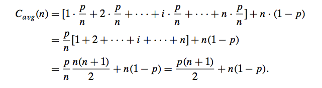
This general formula yields some quite reasonable answers. For example, if p = 1 (the search must be successful), the average number of key comparisons made by sequential search is (n + 1)/2; that is, the algorithm will inspect, on average, about half of the list’s elements. If p = 0 (the search must be unsuccessful), the average number of key comparisons will be n because the algorithm will inspect all n elements on all such inputs.
Time–Space Trade-off
The best algorithm to solve a particular problem at hand is no doubt the one that requires less memory space and takes less time to complete its execution. But practically, designing such an ideal algorithm is not a trivial task. There can be more than one algorithm to solve a particular problem. One may require less memory space, while the other may require less CPU time to execute. Thus, it is not uncommon to sacrifice one thing for the other. Hence, there exists a time–space trade-off among algorithms.
So, if space is a big constraint, then one might choose a program that takes less space at the cost of more CPU time. On the contrary, if time is a major constraint, then one might choose a program that takes minimum time to execute at the cost of more space.
Expressing Time and Space Complexity
The time and space complexity can be expressed using a function f(n) where n is the input size for a given instance of the problem being solved. Expressing the complexity is required when
- We want to predict the rate of growth of complexity as the input size of the problem increases.
- There are multiple algorithms that find a solution to a given problem and we need to find the algorithm that is most efficient.
The most widely used notation to express this function f(n) is the Big O notation. It provides the upper bound for the complexity.
Algorithm Efficiency
If a function is linear (without any loops or recursions), the efficiency of that algorithm or the running time of that algorithm can be given as the number of instructions it contains. However, if an algorithm contains loops, then the efficiency of that algorithm may vary depending on the number of loops and the running time of each loop in the algorithm.
Let us consider different cases in which loops determine the efficiency of an algorithm.
Linear Loops
To calculate the efficiency of an algorithm that has a single loop, we need to first determine the number of times the statements in the loop will be executed. This is because the number of iterations is directly proportional to the loop factor. Greater the loop factor, more is the number of iterations. For example, consider the loop given below:
for(i=0;i<100;i++) statement block;
Here, 100 is the loop factor. We have already said that efficiency is directly proportional to the number of iterations. Hence, the general formula in the case of linear loops may be given as
f(n) = n
However calculating efficiency is not as simple as is shown in the above example. Consider the loop given below:
for(i=0;i<100;i+=2) statement block;
Here, the number of iterations is half the number of the loop factor. So, here the efficiency can be given as
f(n) = n/2
Logarithmic Loops
We have seen that in linear loops, the loop updation statement either adds or subtracts the loop-controlling variable. However, in logarithmic loops, the loop-controlling variable is either multiplied or divided during each iteration of the loop. For example, look at the loops given below:
for(i=1;i<1000;i*=2)                      for(i=1000;i>=1;i/=2)

     statement block;                                    statement block;
Consider the first for loop in which the loop-controlling variable i is multiplied by 2. The loop will be executed only 10 times and not 1000 times because in each iteration the value of i doubles. Now, consider the second loop in which the loop-controlling variable i is divided by 2. In this case also, the loop will be executed 10 times. Thus, the number of iterations is a function of the number by which the loop-controlling variable is divided or multiplied. In the examples discussed, it is 2. That is, when n = 1000, the number of iterations can be given by log 1000 which is approximately equal to 10.
Therefore, putting this analysis in general terms, we can conclude that the efficiency of loops in which iterations divide or multiply the loop-controlling variables can be given as
f(n) = log n
Nested Loops
Loops that contain loops are known as nested loops. In order to analyze nested loops, we need to determine the number of iterations each loop completes. The total is then obtained as the product of the number of iterations in the inner loop and the number of iterations in the outer loop.
In this case, we analyze the efficiency of the algorithm based on whether it is a linear logarithmic, quadratic, or dependent quadratic nested loop.
Linear logarithmic loop
Consider the following code in which the loop-controlling variable of the inner loop is multiplied after each iteration. The number of iterations in the inner loop is log 10. This inner loop is controlled by an outer loop which iterates 10 times. Therefore, according to the formula, the number of iterations for this code can be given as 10 log 10.
for(i=0;i<10;i++)

   for(j=1; j<10;j*=2)

       statement block;
In more general terms, the efficiency of such loops can be given as f(n) = n log n.
Quadratic loop
In a quadratic loop, the number of iterations in the inner loop is equal to the number of iterations in the outer loop. Consider the following code in which the outer loop executes 10 times and for each iteration of the outer loop, the inner loop also executes 10 times. Therefore, the efficiency here is 100.
for(i=0;i<10;i++)

   for(j=0; j<10;j++)

       statement block;
The generalized formula for quadratic loop can be given as f(n) = n^2.
Dependent quadratic loop
In a dependent quadratic loop, the number of iterations in the inner loop is dependent on the outer loop. Consider the code given below:
 for(i=0;i<10;i++)

for(j=0; j<=i;j++)

     statement block;
In this code, the inner loop will execute just once in the first iteration, twice in the second iteration, thrice in the third iteration, so on and so forth. In this way, the number of iterations can be calculated as
1 + 2 + 3 + ... + 9 + 10 = 55
If we calculate the average of this loop (55/10 = 5.5), we will observe that it is equal to the number of iterations in the outer loop (10) plus 1 divided by 2. In general terms, the inner loop iterates (n + 1)/2 times. Therefore, the efficiency of such a code can be given as
f(n) = n (n + 1)/2