Introduction: data types, data structures and abstract data types

Introduction

A data structure is a way of organizing and storing data in a computer so that it can be used efficiently. It defines a particular way of organizing data in a computer's memory and provides operations to manipulate that data. Essentially, it's about organizing, managing, and storing data in a way that facilitates efficient access and modification.

How computer programming uses data structures?

A program should undoubtedly give correct results, but along with that it should also run efficiently. A program is said to be efficient when it executes in minimum time and with minimum memory space. 

In order to write efficient programs, we need to apply certain data management concepts. The concept of data management is a complex task that includes activities like data collection, organization of data into appropriate structures, and developing and maintaining routines for quality assurance. 

Data structure is a crucial part of data management. A data structure is basically a group of data elements that are put together under one name, and which defines a particular way of storing and organizing data in a computer so that it can be used efficiently.

Data structures are fundamental in programming for several reasons:

• Efficient Data Organization: Different data structures are optimized for different operations. For example, arrays are efficient for random access, while linked lists are efficient for insertions and deletions.
• Optimized Algorithms: Many algorithms rely on specific data structures to achieve efficiency. Using the appropriate data structure can significantly improve the performance of algorithms.
• Memory Management: Data structures help in efficient memory management by allocating and deallocating memory as needed.
• Abstraction: Data structures provide an abstraction layer, hiding the implementation details from the user and allowing them to focus on solving problems at a higher level.

Real-World Scenarios and its use cases

Data structures are used in almost every program or software system. Some common examples of data structures are arrays, linked lists, queues, stacks, binary trees, and hash tables. Data structures are widely applied in the following areas: 

• Compiler design 
• Operating system 
• Statistical analysis package 
• DBMS 
• Numerical analysis 
• Simulation 
• Artificial intelligence 
• Graphics 

When you will study DBMS as a subject, you will realize that the major data structures used in the Network data model are graphs, Hierarchical data model is trees, and RDBMS is arrays. 

Specific data structures are essential ingredients of many efficient algorithms as they enable the programmers to manage huge amounts of data easily and efficiently. Some formal design methods and programming languages emphasize data structures and the algorithms as the key organizing factor in software design. This is because representing information is fundamental to computer science. The primary goal of a program or software is not to perform calculations or operations but to store and retrieve information as fast as possible.

Data structures are used extensively in various real-world scenarios, including:

• Databases: Data structures like B-trees and hash tables are used in databases for efficient storage and retrieval of data.
• Operating Systems: Data structures such as queues and stacks are used in operating systems for managing processes, scheduling tasks, and handling interrupts.
• Network Routing: Graph data structures are used in network routing algorithms to find the shortest path between two nodes in a network.
• Web Development: Data structures like trees and hash maps are used in web development for representing HTML DOM structures and managing session data.

When selecting a data structure to solve a problem, the following steps must be performed. 

• Analysis of the problem to determine the basic operations that must be supported. For example, basic operation may include inserting/deleting/searching a data item from the data structure. 
• Quantify the resource constraints for each operation. 
• Select the data structure that best meets these requirements

Classification of data structure

Data structures are generally categorized into two classes: primitive and non-primitive data structures.

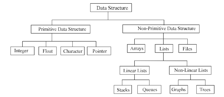
Primitive and Non-primitive Data Structures 

Primitive data structures are the fundamental data types which are supported by a programming language. Some basic data types are integer, real, character, and Boolean. The terms ‘data type’, ‘basic data type’, and ‘primitive data type’ are often used interchangeably. 

Non-primitive data structures are those data structures which are created using primitive data structures. Examples of such data structures include linked lists, stacks, trees, and graphs.

Non-primitive data structures can further be classified into two categories: linear and non-linear data structures.

Linear and Non-linear Structures 

If the elements of a data structure are stored in a linear or sequential order, then it is a linear data structure. Examples include arrays, linked lists, stacks, and queues. Linear data structures can be represented in memory in two different ways. One way is to have a linear relationship between elements by means of sequential memory locations. The other way is to have a linear relationship between elements by means of links.

However, if the elements of a data structure are not stored in a sequential order, then it is a non-linear data structure. The relationship of adjacency is not maintained between elements of a non-linear data structure. Examples include trees and graphs.

Arrays

An array is a collection of similar data elements. These data elements have the same data type. The elements of the array are stored in consecutive memory locations and are referenced by an index (also known as the subscript). 

In C, arrays are declared using the following syntax: 

type name[size]; 

For example, 

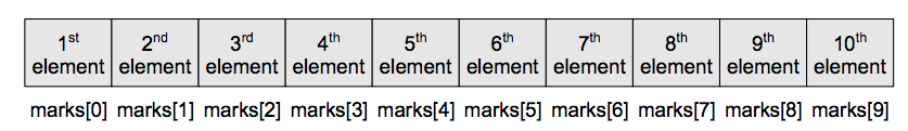
int marks[10];

The above statement declares an array mark that contains 10 elements. In C, the array index starts from zero. This means that the array marks will contain 10 elements in all. The first element will be stored in marks[0], second element in marks[1], so on and so forth. Therefore, the last element, that is the 10th element, will be stored in marks[9]. In the memory, the array will be stored as shown in Figure below:

Arrays are generally used when we want to store large amount of similar type of data. But they have the following limitations: 

• Arrays are of fixed size. 
• Data elements are stored in contiguous memory locations which may not be always available.
• Insertion and deletion of elements can be problematic because of shifting of elements from their positions.

Linked Lists 

A linked list is a very flexible, dynamic data structure in which elements (called nodes) form a sequential list. In contrast to static arrays, a programmer need not worry about how many elements will be stored in the linked list. This feature enables the programmers to write robust programs which require less maintenance. In a linked list, each node is allocated space as it is added to the list. Every node in the list points to the next node in the list. Therefore, in a linked list, every node contains the following two types of data:

• The value of the node or any other data that corresponds to that node 
• A pointer or link to the next node in the list

The last node in the list contains a NULL pointer to indicate that it is the end or tail of the list. Since the memory for a node is dynamically allocated when it is added to the list, the total number of nodes that may be added to a list is limited only by the amount of memory available.

Stacks 

A stack is a linear data structure in which insertion and deletion of elements are done at only one end, which is known as the top of the stack. Stack is called a last-in, first-out (LIFO) structure because the last element which is added to the stack is the first element which is deleted from the stack. 

In the computer’s memory, stacks can be implemented using arrays or linked lists. Figure below shows the array implementation of a stack. Every stack has a variable top associated with it. top is used to store the address of the topmost element of the stack. It is this position from where the element will be added or deleted. There is another variable MAX, which is used to store the maximum number of elements that the stack can store. 

If top = NULL, then it indicates that the stack is empty and if top = MAX–1, then the stack is full.

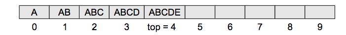
In Figure above, top = 4, so insertions and deletions will be done at this position. Here, the stack can store a maximum of 10 elements where the indices range from 0–9. In the above stack, five more elements can still be stored. 

A stack supports three basic operations: push, pop, and peep. The push operation adds an element to the top of the stack. The pop operation removes the element from the top of the stack. And the peep operation returns the value of the topmost element of the stack (without deleting it). 

However, before inserting an element in the stack, we must check for overflow conditions. An overflow occurs when we try to insert an element into a stack that is already full. Similarly, before deleting an element from the stack, we must check for underflow conditions. An underflow condition occurs when we try to delete an element from a stack that is already empty.

Queue

A queue is a first-in, first-out (FIFO) data structure in which the element that is inserted first is the first one to be taken out. The elements in a queue are added at one end called the rear and removed from the other end called the front. Like stacks, queues can be implemented by using either arrays or linked lists. Every queue has front and rear variables that point to the position from where deletions and insertions can be done, respectively. Consider the queue shown in Figure below:

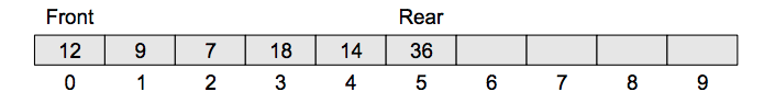
Fig. Array representation of queue

Here, front = 0 and rear = 5. If we want to add one more value to the list, say, if we want to add another element with the value 45, then the rear would be incremented by 1 and the value would be stored at the position pointed by the rear. The queue, after the addition, would be as shown in Figure below:

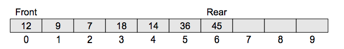
Fig. Queue after insertion of new elements

 Here, front = 0 and rear = 6. Every time a new element is to be added, we will repeat the same procedure.

Now, if we want to delete an element from the queue, then the value of front will be incremented. Deletions are done only from this end of the queue. The queue after the deletion will be as shown in Figure below:

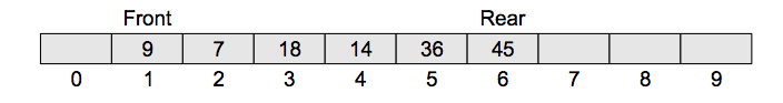
Fig. Queue after deletion of element

However, before inserting an element in the queue, we must check for overflow conditions. An overflow occurs when we try to insert an element into a queue that is already full. A queue is full when rear = MAX–1, where MAX is the size of the queue, that is MAX specifies the maximum number of elements in the queue. Note that we have written MAX–1 because the index starts from 0. 

Similarly, before deleting an element from the queue, we must check for underflow conditions. An underflow condition occurs when we try to delete an element from a queue that is already empty. If front = NULL and rear = NULL, then there is no element in the queue.

Trees 

A tree is a non-linear data structure which consists of a collection of nodes arranged in a hierarchical order. One of the nodes is designated as the root node, and the remaining nodes can be partitioned into disjoint sets such that each set is a subtree of the root. 

The simplest form of a tree is a binary tree. A binary tree consists of a root node and left and right subtrees, where both sub-trees are also binary trees. Each node contains a data element, a left pointer which points to the left sub-tree, and a right pointer which points to the right subtree. The root element is the topmost node which is pointed by a ‘root’ pointer. If root = NULL then the tree is empty. 

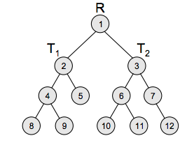
Figure above shows a binary tree, where R is the root node and T1 and T2 are the left and right subtrees of R. If T1 is non-empty, then T1 is said to be the left successor of R. Likewise, if T2 is non-empty, then it is called the right successor of R.

Graph

A graph is a non-linear data structure which is a collection of vertices (also called nodes) and edges that connect these vertices. A graph is often viewed as a generalization of the tree structure, where instead of a purely parent-to-child relationship between tree nodes, any kind of complex relationships between the nodes can exist. 

In a tree structure, nodes can have any number of children but only one parent, a graph on the other hand relaxes all such kinds of restrictions. Figure below shows a graph with five nodes. 

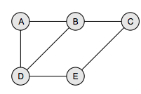
A node in the graph may represent a city and the edges connecting the nodes can represent roads. A graph can also be used to represent a computer network where the nodes are workstations and the edges are the network connections. Graphs have so many applications in computer science and mathematics that several algorithms have been written to perform the standard graph operations, such as searching the graph and finding the shortest path between the nodes of a graph. Note that unlike trees, graphs do not have any root node. Rather, every node in the graph can be connected with another node in the graph. When two nodes are connected via an edge, the two nodes are known as neighbors. For example, in Figure above node A has two neighbors: B and D.

Operations on data structures

• Traversing It means to access each data item exactly once so that it can be processed. For example, to print the names of all the students in a class. 
• Searching It is used to find the location of one or more data items that satisfy the given constraint. Such a data item may or may not be present in the given collection of data items. For example, to find the names of all the students who secured 100 marks in mathematics. 
• Inserting It is used to add new data items to the given list of data items. For example, to add the details of a new student who has recently joined the course.
• Deleting It means to remove (delete) a particular data item from the given collection of data items. For example, to delete the name of a student who has left the course. 
• Sorting Data items can be arranged in some order like ascending order or descending order depending on the type of application. For example, arranging the names of students in a class in an alphabetical order, or calculating the top three winners by arranging the participants’ scores in descending order and then extracting the top three. 
• Merging Lists of two sorted data items can be combined to form a single list of sorted data items.

ABSTRACT DATA TYPE (ADT)

An abstract data type (ADT) is the way we look at a data structure, focusing on what it does and ignoring how it does its job. For example, stacks and queues are perfect examples of an ADT. We can implement both these ADTs using an array or a linked list. This demonstrates the ‘abstract’ nature of stacks and queues. To further understand the meaning of an abstract data type, we will break the term into ‘data type’ and ‘abstract’, and then discuss their meanings.

Data type 

Data type of a variable is the set of values that the variable can take. We have already read the basic data types in C include int, char, float, and double. When we talk about a primitive type (built-in data type), we actually consider two things: a data item with certain characteristics and the permissible operations on that data. 

For example, an int variable can contain any whole-number value from –32768 to 32767 and can be operated with the operators +, –, *, and /. In other words, the operations that can be performed on a data type are an inseparable part of its identity. Therefore, when we declare a variable of an abstract data type (e.g., stack or a queue), we also need to specify the operations that can be performed on it. 

Abstract 

The word ‘abstract’ in the context of data structures means considered apart from the detailed specifications or implementation. In C, an abstract data type can be a structure considered without regard to its implementation. It can be thought of as a ‘description’ of the data in the structure with a list of operations that can be performed on the data within that structure. 

The end-user is not concerned about the details of how the methods carry out their tasks. They are only aware of the methods that are available to them and are only concerned about calling those methods and getting the results. They are not concerned about how they work. 

For example, when we use a stack or a queue, the user is concerned only with the type of data and the operations that can be performed on it. Therefore, the fundamentals of how the data is stored should be invisible to the user. They should not be concerned with how the methods work or what structures are being used to store the data. They should just know that to work with stacks, they have push() and pop() functions available to them. Using these functions, they can manipulate the data (insertion or deletion) stored in the stack.

Algorithms

Algorithm is ‘a formally defined procedure for performing some calculation’. If a procedure is formally defined, then it can be implemented using a formal language, and such a language is known as a programming language. In general terms, an algorithm provides a blueprint to write a program to solve a particular problem. It is considered to be an effective procedure for solving a problem in finite number of steps. That is, a well-defined algorithm always provides an answer and is guaranteed to terminate. 

Algorithms are mainly used to achieve software reuse. Once we have an idea or a blueprint of a solution, we can implement it in any high-level language like C, C++, or Java. 

An algorithm is basically a set of instructions that solve a problem. It is not uncommon to have multiple algorithms to tackle the same problem, but the choice of a particular algorithm must depend on the time and space complexity of the algorithm.

DIFFERENT APPROACHES TO DESIGNING AN ALGORITHM 

Algorithms are used to manipulate the data contained in data structures. When working with data structures, algorithms are used to perform operations on the stored data. 

A complex algorithm is often divided into smaller units called modules. This process of dividing an algorithm into modules is called modularization. The key advantages of modularization are as follows: 

It makes the complex algorithm simpler to design and implement.

Each module can be designed independently. While designing one module, the details of other modules can be ignored, thereby enhancing clarity in design which in turn simplifies implementation, debugging, testing, documenting, and maintenance of the overall algorithm. 

There are two main approaches to design an algorithm—top-down approach and bottom-up approach, as shown in Figure below: -

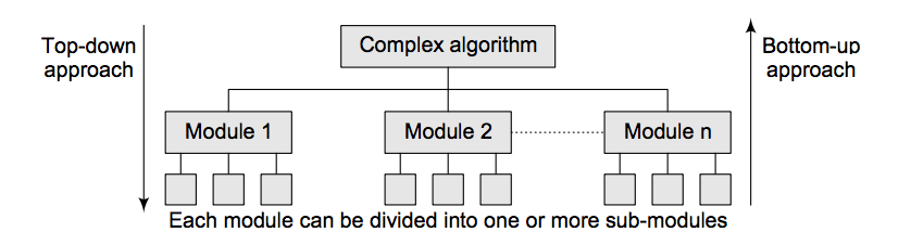
Fig. Different approaches of designing an algorithm

Top-down approach A top-down design approach starts by dividing the complex algorithm into one or more modules. These modules can further be decomposed into one or more sub-modules, and this process of decomposition is iterated until the desired level of module complexity is achieved. Top-down design method is a form of stepwise refinement where we begin with the topmost module and incrementally add modules that it calls. 

Therefore, in a top-down approach, we start from an abstract design and then at each step, this design is refined into more concrete levels until a level is reached that requires no further refinement. 

Bottom-up approach A bottom-up approach is just the reverse of top-down approach. In the bottom-up design, we start with designing the most basic or concrete modules and then proceed towards designing higher level modules. The higher level modules are implemented by using the operations performed by lower level modules. Thus, in this approach sub-modules are grouped together to form a higher level module. All the higher level modules are clubbed together to form even higher level modules. This process is repeated until the design of the complete algorithm is obtained.

CONTROL STRUCTURES USED IN ALGORITHMS 

An algorithm has a finite number of steps. Some steps may involve decision-making and repetition. Broadly speaking, an algorithm may employ one of the following control structures: (a) sequence, (b) decision, and (c) repetition.

Sequence 

By sequence, we mean that each step of an algorithm is executed in a specified order. Let us write an algorithm to add two numbers. This algorithm performs the steps in a purely sequential order, as shown below :-

Step 1 : Input first number as A

Step 2 : Input second number as B

Step 3 :  Set SUM = A+B

Step 4 : print SUM

Step 5 : END

Decision 

Decision statements are used when the execution of a process depends on the outcome of some condition. 

A decision statement can also be stated in the following manner: 

IF condition
              Then process1 

ELSE         process2

Example:

Step 1 : Input first number as A

Step 2 : Input second number as B

Step 3 :  IF  A=B

                    Print “EQUAL”

              ELSE

                    Print “NOT EQUAL”

             [END of IF]

Step 5 : END

Repetition, which involves executing one or more steps for a number of times, can be implemented using constructs such as while, do–while, and for loops. These loops execute one or more steps until some condition is true.

Step 1: [INITIALIZE] set I=1, N=10

Step 2: Repeat step 3 and 4 WHILE I<=N

Step 3: PRINT I, set I=I+1

            [END of LOOP]

Step 4: END

TIME AND SPACE COMPLEXITY 

Analyzing an algorithm means determining the amount of resources (such as time and memory) needed to execute it. Algorithms are generally designed to work with an arbitrary number of inputs, so the efficiency or complexity of an algorithm is stated in terms of time and space complexity. 

The time complexity of an algorithm is basically the running time of a program as a function of the input size. Similarly, the space complexity of an algorithm is the amount of computer memory that is required during the program execution as a function of the input size. 

In other words, the number of machine instructions which a program executes is called its time complexity. This number is primarily dependent on the size of the program’s input and the algorithm used. 

Generally, the space needed by a program depends on the following two parts: 

Fixed part: It varies from problem to problem. It includes the space needed for storing instructions, constants, variables, and structured variables (like arrays and structures). 

Variable part: It varies from program to program. It includes the space needed for recursion stack, and for structured variables that are allocated space dynamically during the runtime of a program.
However, running time requirements are more critical than memory requirements. Therefore, we will concentrate on the running time efficiency of algorithms.

Worst-Case, Best-Case, and Average-Case Efficiencies

We have established that it is reasonable to measure an algorithm’s efficiency as a function of a parameter indicating the size of the algorithm’s input. But there are many algorithms for which running time depends not only on an input size but also on the specifics of a particular input. 

Consider, as an example, sequential search. This is a straightforward algorithm that searches for a given item (some search key K) in a list of n elements by checking successive elements of the list until either a match with the search key is found or the list is exhausted. 

Here is the algorithm’s pseudocode, in which, for simplicity, a list is implemented as an array. 

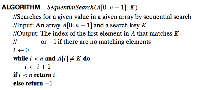
Clearly, the running time of this algorithm can be quite different for the same list size n. In the worst case, when there are no matching elements or the first matching element happens to be the last one on the list, the algorithm makes the largest number of key comparisons among all possible inputs of size n: C_worst(n) = n.

The worst-case efficiency of an algorithm is its efficiency for the worst-case input of size n, which is an input (or inputs) of size n for which the algorithm runs the longest among all possible inputs of that size. The way to determine the worst-case efficiency of an algorithm is, in principle, quite straightforward: analyze the algorithm to see what kind of inputs yield the largest value of the basic operation’s count C(n) among all possible inputs of size n and then compute this worst-case value C_worst(n).  

The best-case efficiency of an algorithm is its efficiency for the best-case input of size n, which is an input (or inputs) of size n for which the algorithm runs the fastest among all possible inputs of that size. Accordingly, we can analyze the best- case efficiency as follows. First, we determine the kind of inputs for which the count C(n) will be the smallest among all possible inputs of size n. (Note that the best case does not mean the smallest input; it means the input of size n for which the algorithm runs the fastest.) Then we ascertain the value of C(n) on these most convenient inputs. For example, the best-case inputs for sequential search are lists of size n with their first element equal to a search key; accordingly, Cbest (n) = 1 for this algorithm. 

The analysis of the best-case efficiency is not nearly as important as that of the worst-case efficiency. But it is not completely useless, either. Though we should not expect to get best-case inputs, we might be able to take advantage of the fact that for some algorithms a good best-case performance extends to some useful types of inputs close to being the best-case ones. For example, there is a sorting algorithm (insertion sort) for which the best-case inputs are already sorted arrays on which the algorithm works very fast. Moreover, the best-case efficiency deteriorates only slightly for almost-sorted arrays. Therefore, such an algorithm might well be the method of choice for applications dealing with almost-sorted arrays. And, of course, if the best-case efficiency of an algorithm is unsatisfactory, we can immediately discard it without further analysis.

It should be clear from our discussion, however, that neither the worst-case analysis nor its best-case counterpart yields the necessary information about an algorithm’s behavior on a “typical” or “random” input. This is the information that the average-case efficiency seeks to provide. To analyze the algorithm’s average- case efficiency, we must make some assumptions about possible inputs of size n. 

Let’s consider again sequential search. The standard assumptions are that : 

(a) the probability of a successful search is equal to p (0 ≤ p ≤ 1) and 

(b) the probability of the first match occurring in the ith position of the list is the same for every i. 

Under these assumptions—the validity of which is usually difficult to verify, their reasonableness notwithstanding—we can find the average number of key comparisons Cavg(n) as follows. 

In the case of a successful search, the probability of the first match occurring in the ith position of the list is p/n for every i, and the number of comparisons made by the algorithm in such a situation is obviously i. In the case of an unsuccessful search, the number of comparisons will be n with the probability of such a search being (1 − p). Therefore, 

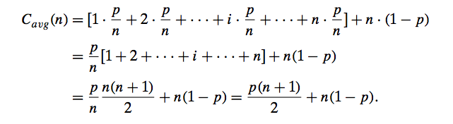
This general formula yields some quite reasonable answers. For example, if p = 1 (the search must be successful), the average number of key comparisons made by sequential search is (n + 1)/2; that is, the algorithm will inspect, on average, about half of the list’s elements. If p = 0 (the search must be unsuccessful), the average number of key comparisons will be n because the algorithm will inspect all n elements on all such inputs.  

Time–Space Trade-off 

The best algorithm to solve a particular problem at hand is no doubt the one that requires less memory space and takes less time to complete its execution. But practically, designing such an ideal algorithm is not a trivial task. There can be more than one algorithm to solve a particular problem. One may require less memory space, while the other may require less CPU time to execute. Thus, it is not uncommon to sacrifice one thing for the other. Hence, there exists a time–space trade-off among algorithms. 

So, if space is a big constraint, then one might choose a program that takes less space at the cost of more CPU time. On the contrary, if time is a major constraint, then one might choose a program that takes minimum time to execute at the cost of more space.

Expressing Time and Space Complexity 

The time and space complexity can be expressed using a function f(n) where n is the input size for a given instance of the problem being solved. Expressing the complexity is required when 

• We want to predict the rate of growth of complexity as the input size of the problem increases.
• There are multiple algorithms that find a solution to a given problem and we need to find the algorithm that is most efficient. 

The most widely used notation to express this function f(n) is the Big O notation. It provides the upper bound for the complexity.

Algorithm Efficiency 

If a function is linear (without any loops or recursions), the efficiency of that algorithm or the running time of that algorithm can be given as the number of instructions it contains. However, if an algorithm contains loops, then the efficiency of that algorithm may vary depending on the number of loops and the running time of each loop in the algorithm. 

Let us consider different cases in which loops determine the efficiency of an algorithm.

Linear Loops 

To calculate the efficiency of an algorithm that has a single loop, we need to first determine the number of times the statements in the loop will be executed. This is because the number of iterations is directly proportional to the loop factor. Greater the loop factor, more is the number of iterations. For example, consider the loop given below: 

for(i=0;i<100;i++)          statement block; 

Here, 100 is the loop factor. We have already said that efficiency is directly proportional to the number of iterations. Hence, the general formula in the case of linear loops may be given as 

f(n) = n 

However calculating efficiency is not as simple as is shown in the above example. Consider the loop given below: 

for(i=0;i<100;i+=2)           statement block; 

Here, the number of iterations is half the number of the loop factor. So, here the efficiency can be given as 

f(n) = n/2

Logarithmic Loops 

We have seen that in linear loops, the loop updation statement either adds or subtracts the loop-controlling variable. However, in logarithmic loops, the loop-controlling variable is either multiplied or divided during each iteration of the loop. For example, look at the loops given below: 

for(i=1;i<1000;i*=2)                      for(i=1000;i>=1;i/=2) 

     statement block;                                    statement block; 

Consider the first for loop in which the loop-controlling variable i is multiplied by 2. The loop will be executed only 10 times and not 1000 times because in each iteration the value of i doubles. Now, consider the second loop in which the loop-controlling variable i is divided by 2. In this case also, the loop will be executed 10 times. Thus, the number of iterations is a function of the number by which the loop-controlling variable is divided or multiplied. In the examples discussed, it is 2. That is, when n = 1000, the number of iterations can be given by log 1000 which is approximately equal to 10. 

Therefore, putting this analysis in general terms, we can conclude that the efficiency of loops in which iterations divide or multiply the loop-controlling variables can be given as 

f(n) = log n

Nested Loops 

Loops that contain loops are known as nested loops. In order to analyze nested loops, we need to determine the number of iterations each loop completes. The total is then obtained as the product of the number of iterations in the inner loop and the number of iterations in the outer loop. 

In this case, we analyze the efficiency of the algorithm based on whether it is a linear logarithmic, quadratic, or dependent quadratic nested loop. 

Linear logarithmic loop 

Consider the following code in which the loop-controlling variable of the inner loop is multiplied after each iteration. The number of iterations in the inner loop is log 10. This inner loop is controlled by an outer loop which iterates 10 times. Therefore, according to the formula, the number of iterations for this code can be given as 10 log 10. 

for(i=0;i<10;i++)      

   for(j=1; j<10;j*=2)                        

       statement block; 

In more general terms, the efficiency of such loops can be given as f(n) = n log n. 

Quadratic loop 

In a quadratic loop, the number of iterations in the inner loop is equal to the number of iterations in the outer loop. Consider the following code in which the outer loop executes 10 times and for each iteration of the outer loop, the inner loop also executes 10 times. Therefore, the efficiency here is 100. 

for(i=0;i<10;i++)                 

   for(j=0; j<10;j++) 

       statement block;
 

The generalized formula for quadratic loop can be given as f(n) = n^2. 

Dependent quadratic loop 

In a dependent quadratic loop, the number of iterations in the inner loop is dependent on the outer loop. Consider the code given below: 

 for(i=0;i<10;i++)                 

for(j=0; j<=i;j++)                        

     statement block;

 In this code, the inner loop will execute just once in the first iteration, twice in the second iteration, thrice in the third iteration, so on and so forth. In this way, the number of iterations can be calculated as 

1 + 2 + 3 + ... + 9 + 10 = 55 

If we calculate the average of this loop (55/10 = 5.5), we will observe that it is equal to the number of iterations in the outer loop (10) plus 1 divided by 2. In general terms, the inner loop iterates (n + 1)/2 times. Therefore, the efficiency of such a code can be given as 

f(n) = n (n + 1)/2