Collision in Hash Table

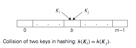
if we choose a hash table’s size m to be smaller than the number of keys n, we will get collisions—a phenomenon of two (or more) keys being hashed into the same cell of the hash table as shown above. But collisions should be expected even if m is considerably larger than n. In fact, in the worst case, all the keys could be hashed to the same cell of the hash table. Fortunately, with an appropriately chosen hash table size and a good hash function, this situation happens very rarely. Still, every hashing scheme must have a collision resolution mechanism. This mechanism is different in the two principal versions of hashing: open hashing (also called separate chaining) and closed hashing (also called open addressing).

Collision Resolution Techniques

When implementing a hash table, collisions are inevitable due to the possibility of multiple keys hashing to the same index in the table. To handle collisions, various collision resolution techniques are employed. The two primary collision resolution techniques are:

• open hashing (also called separate chaining)
• closed hashing (also called open addressing)

Open Hashing (Separate Chaining)

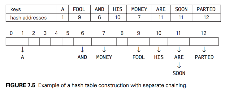
In open hashing, keys are stored in linked lists attached to cells of a hash table. Each list contains all the keys hashed to its cell. Consider, as an example, the following list of words:

A, FOOL, AND, HIS, MONEY, ARE, SOON, PARTED.

As a hash function, we will use the simple function for strings mentioned above, i.e., we will add the positions of a word’s letters in the alphabet and compute the sum’s remainder after division by 13. We start with the empty table. The first key is the word A; its hash value is h(A) = 1 mod 13 = 1. The second key—the word FOOL—is installed in the ninth cell since (6 + 15 + 15 + 12) mod 13 = 9, and so on. The final result of this process is given in Figure below; note a collision of the keys ARE and SOON because h(ARE) = (1 + 18 + 5) mod 13 = 11 and h(SOON) = (19 + 15 + 15 + 14) mod 13 = 11. 

How do we search in a dictionary implemented as such a table of linked lists? We do this by simply applying to a search key the same procedure that was used for creating the table. To illustrate, if we want to search for the key KID in the hash table of Figure 7.5, we first compute the value of the same hash function for the key: h(KID) = 11. Since the list attached to cell 11 is not empty, its linked list may contain the search key. But because of possible collisions, we cannot tell whether this is the case until we traverse this linked list. After comparing the string KID first with the string ARE and then with the string SOON, we end up with an unsuccessful search.

Insertions are normally done at the end of a list. Deletion is performed by searching for a key to be deleted and then removing it from its list.

Closed Hashing (Open Addressing)

In closed hashing, all keys are stored in the hash table itself without the use of linked lists. (Of course, this implies that the table size m must be at least as large as the number of keys n.) Different strategies can be employed for collision resolution. The simplest one—called linear probing—checks the cell following the one where the collision occurs. If that cell is empty, the new key is installed there; if the next cell is already occupied, the availability of that cell’s immediate successor is checked, and so on. Note that if the end of the hash table is reached,

the search is wrapped to the beginning of the table; i.e., it is treated as a circular array. This method is illustrated in Figure below with the same word list and hash function used above to illustrate separate chaining.

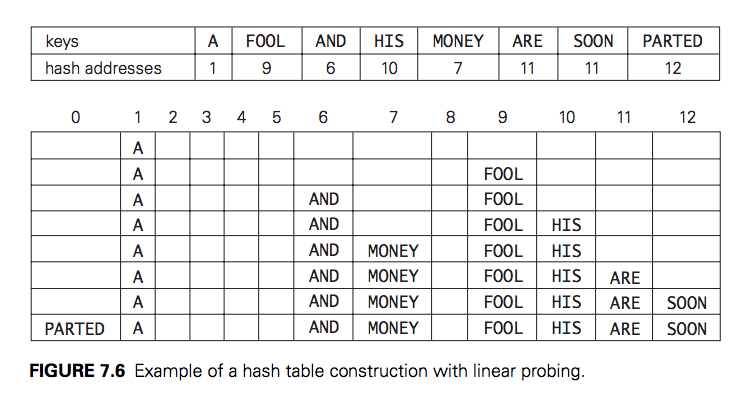
Although the search and insertion operations are straightforward for this version of hashing, deletion is not. For example, if we simply delete the key ARE from the last state of the hash table in Figure above, we will be unable to find the key SOON afterward. Indeed, after computing h(SOON) = 11, the algorithm would find this location empty and report the unsuccessful search result. A simple solution is to use “lazy deletion,” i.e., to mark previously occupied locations by a special symbol to distinguish them from locations that have not been occupied.

Linear Probing:

Linear probing is a simple and commonly used technique for collision resolution in hash tables. When a collision occurs, meaning a key hashes to a slot that is already occupied, linear probing searches for the next available slot in a linear sequence until an empty slot is found.

Algorithm:

1. Compute the hash code of the key to determine its initial position in the hash table.

2. If the slot at the computed index is empty, insert the key-value pair into that slot.

3. If the slot is occupied:

      Start probing linearly from the next slot (index + 1).

      Repeat this process until an empty slot is found.

4. Once an empty slot is found, insert the key-value pair into that slot.