DATABASE MANAGEMENT SYSTEM

Hashing, Static Hashing and Dynamic Hashing 

 

Hashing

 

Hashing is a technique used in database management systems (DBMS) to quickly locate a data record given its search key. This method transforms a search key into an address in the hash table using a hash function. Hashing is highly efficient for queries that involve exact matches and is widely used in applications such as indexing, cache retrieval, and hash joins in databases.The hashing technique utilizes an auxiliary hash table to store the data records using a hash function.

 

Components of Hashing 

 

1. Hash Function

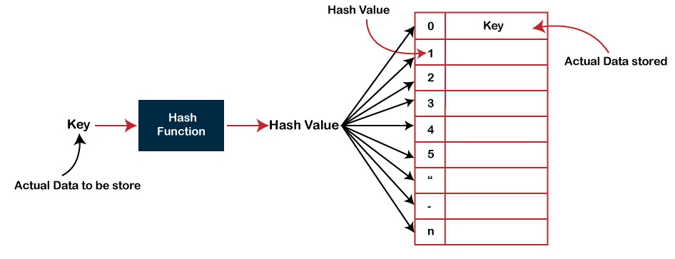
A hash function is a mathematical algorithm that converts an input (or 'key') into a fixed-size string of bytes. The output, typically called a hash code, is used as an index into an array (hash table) where the actual data is stored.

Characteristics:

• The same input key always produces the same hash code.
• A good hash function distributes hash codes uniformly across the hash table to minimize collisions.

2. Hash Table

A hash table is an array-like data structure where data is stored. Each slot in the hash table is called a "bucket" or "slot," and it can store one or more records.

Characteristics:

• The number of slots (or buckets) in the hash table, often denoted as 'n'.
• Hash tables can be either of fixed size (static) or capable of resizing (dynamic).

3. Buckets

Buckets are the individual storage locations within a hash table where records are stored.

Characteristics:

• Each bucket can store one record, typical in open addressing.
• Each bucket can store multiple records, often implemented using linked lists or other structures in chaining.

 

 

Methods of Hashing

 

1. Direct Hashing

Direct hashing assigns a unique hash value to each key without any computation. This method is feasible when the key space is small and manageable.

Example:

• If keys are in the range 0 to 99, each key directly maps to an array index.

2. Modulo Division Hashing

Modulo division hashing uses the remainder of the key divided by the table size as the hash value.

Hash Function: h(k)=kmod  n where k is the key and n is the number of buckets.

Example:

• Key = 123, Table size = 10
• Hash value = 123 % 10 = 3

3. Mid-Square Hashing

Mid-square hashing involves squaring the key and extracting the middle part of the result as the hash value.

Steps:

1. Square the key.
2. Extract the middle part of the squared value.

Example:

• Key = 56
• Squared value = 3136
• Extract middle digits (13) as the hash value.

4. Folding Hashing

Folding hashing divides the key into equal parts, adds these parts together, and uses the result modulo the table size as the hash value.

Steps:

1. Divide the key into equal parts.
2. Add the parts together.
3. Apply modulo operation with the table size.

Example:

• Key = 987654
• Divide into parts: 98, 76, 54
• Sum = 98 + 76 + 54 = 228
• Hash value = 228 % 10 = 8

 

Types of Hashing

 

 

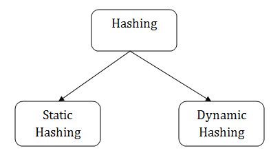
1. Static Hashing 

 

Static hashing is a database management technique in which a fixed-size hash table is used to map keys to data records using a hash function. The hash table size and structure remain constant, irrespective of the number of records stored. This means that the number of buckets or slots available for data storage does not change dynamically, even if the database grows or shrinks over time.

 

Hash Function: A hash function h is used to map a key (e.g., a database record identifier) to a bucket index. The function should distribute keys uniformly across the buckets to minimize collisions (i.e., multiple keys hashing to the same bucket).

 

Buckets: These are the storage units that hold the records. In static hashing, the number of buckets is fixed at the time of creation and does not change dynamically.

Collisions: When two keys hash to the same bucket, a collision occurs. Static hashing must handle collisions using techniques like chaining (linked lists) or open addressing (probing).

 

Working of Static Hashing

1. Initialization: Determine the number of buckets (let’s say N). Choose a hash function that maps keys to an index between 0 and N-1.
2. Insertion:
   • Apply the hash function to the key to get a bucket index.
   • Place the record in the corresponding bucket. If the bucket already contains records, handle the collision using the chosen method (e.g., chaining).
3. Search:
   • Apply the hash function to the key to get the bucket index.
   • Search within the bucket for the desired record. This search can be linear or use more sophisticated structures like binary search if the bucket is kept sorted.
4. Deletion:
   • Apply the hash function to find the bucket.
   • Search for the record within the bucket and remove it. Adjust any linked list or probing structures accordingly.

Advantages of Static Hashing

1. Simplicity: Easy to implement and understand.
2. Performance: Provides O(1) average time complexity for search, insertion, and deletion operations in ideal conditions.
3. Predictability: Since the number of buckets is fixed, memory allocation can be planned and managed efficiently.

Disadvantages of Static Hashing

1. Fixed Size: The number of buckets is fixed, which can lead to inefficiencies. If the number of records grows significantly, many records will end up in the same bucket, leading to increased search times (collisions).
2. Memory Waste: If the number of records is much smaller than the number of buckets, a lot of space may be wasted.
3. Rehashing Complexity: If the hash table becomes too full, rehashing (creating a new, larger hash table and re-inserting all records) can be complex and time-consuming.

Collision Resolution Techniques in Hashing

 

Collision resolution is a critical aspect of hashing because even with a good hash function, collisions (where different keys hash to the same index) are inevitable. 

1. Open Hashing (Chaining)

In Open Hashing, there is a method called Chaining. Chaining makes use of the link list data structure to store the newly added key to the index where the collision occurs. 

How It Works:

• When a collision occurs, the new entry is added to the linked list at that index.
• During lookup, the hash index is found, and the linked list is traversed to find the entry.

Advantages:

• Simple to implement.
• The hash table can accommodate more entries than there are buckets.

Disadvantages:

• Requires additional memory for pointers.
• Performance degrades if many entries hash to the same bucket, leading to long chains.

2. Open Addressing

In open addressing, all entries are stored within the hash table itself. When a collision occurs, the algorithm probes for the next available slot according to a probing sequence.

a. Linear Probing

 In Linear probing the key is added to the next available(empty) index. 

If a collision occurs at index i, the algorithm checks the next slot (i + 1) % table_size, then (i + 2) % table_size, and so on, until an empty slot is found.

Here , i is the probe number or collision number i.e. how many times we attempted for a slot.

Example

Let us consider a hash function h(k)=k mod 10 , with keys 33, 55, 22, 43,79,19,42. Insert in bucket using Linear Probing.

Solution:

The table size will be of 0-(n-1)=0-9

33 mod 10=3—---------33 will go in bucket 3

55 mod 10=5

22 mod 10=2

43 mod 10=3—------here as bucket 3 is already occupied, so collision occur . this can be resolved using Linear Probing.

We apply, h’(K)=(h(k)+i) mod 10

                          =(3+1) mod 10=4 

43 will go in bucket 4

 

Advantages:

• Simple to implement.
• Good cache performance due to locality of reference.

Disadvantages:

• Primary clustering: Long sequences of occupied slots can form(i.e. Probability of an element to go in the same box increases as the data increases), leading to performance degradation.

b. Quadratic Probing

How It Works:

• If a collision occurs at index i, the algorithm checks slots (h(k) + i^2) % table_size, (h(k)+ (i+1)^2) % table_size, and so on.

Example

Let us consider a hash function h(k)=k mod 10 , with keys 42,16,91,33,18,27,36,69. Insert in bucket using Quadratic Probing.

Solution:

The table size will be of 0-(n-1)=0-9

42 mod 10=2—---------42 will go in bucket 2

16 mod 10=6

91 mod 10=1

33 mod 10=3

18 mod 10=8

27 mod 10=7

36 mod 10=6—------here as bucket 6 is already occupied, so collision occur . this can be resolved using Quadratic Probing.

We apply, h’(K,i)=(h(k)+i^2) mod 10

                          =(6+1) mod 10=7—-----here bucket 7 is already occupied , so we increase the value of i to 2

                             =(6+4) mod 10=0

Hence 36 goes to bucket 0 

43 will go in bucket 4

 

Advantages:

• Reduces primary clustering.

Disadvantages:

• Secondary clustering: Different keys that hash to the same initial index follow the same probing sequence.
• More complex than linear probing.

c. Double Hashing

 

In Double Hashing there are two hash functions, Let us consider h1(k) = k mod 11 where n should be prime  and h2(k) = 8-(k mod 8)  where n should be less than n and result is stored in (h1(k) + ih2(k)) mod 11.

 

How It Works:

• Uses a second hash function to calculate the step size for probing.
• If a collision occurs at index i, the next slot is calculated as (i + j * h2(key)) % table_size, where h2 is a second hash function.

Example 

For example, if keys are 20, 34, 45, 70, and 76.

20 mod 11=9

34 mod 11=1

45 mod 11=1  —--------here collision occur so calculate h2(k)

h2(k)=8-(45 mod 8)=8-5=3

(h1(k)+ih2(k))mod 11=(1+1*3)mod 11=4

70 mod 11=4 —----so next slot will be 6(calculate yourself)

56 mod 11=1—-----so next slot will be 3 (calculate yourself)

 

 

Advantages:

• Reduces both primary and secondary clustering.
• Provides a more uniform distribution of probes.

Disadvantages:

• More complex to implement.
• Choosing an appropriate second hash function is crucial.

 

 

2. Dynamic Hashing 

 

Dynamic hashing is an advanced hashing technique used in Database Management Systems (DBMS) to overcome the limitations of static hashing. It allows the hash table to expand and contract dynamically as the number of records grows or shrinks. This adaptability ensures better performance and efficient use of memory.

Extendible Hashing 

 

Extendible hashing is a dynamic hashing technique used in database systems and file systems to handle the problem of hash collisions efficiently and to manage the growth of the dataset. Here’s a comprehensive look at how it works:

Basics of Extendible Hashing

1. Hashing Function:
   • A hashing function is used to compute the hash value of a key. The hash value is a binary number.
2. Directory:
   • The directory is an array of pointers to buckets. Each entry in the directory points to a bucket that can store multiple records.
   • The directory grows dynamically. The size of the directory is a power of 2, and it grows as needed to accommodate more keys.
3. Buckets:
   • Buckets are storage containers for records. Each bucket has a fixed capacity.
   • Each bucket can store multiple key-value pairs.
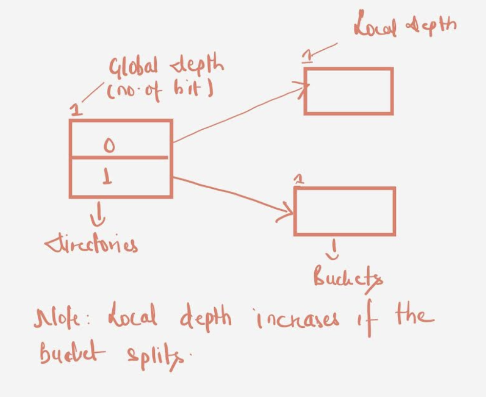
4. Global Depth and Local Depth:
   • Global Depth (GD): The number of bits used from the hash value to index into the directory. As the directory expands, the global depth increases.
   • Local Depth (LD): Each bucket has its own local depth, which represents the number of bits from the hash value used to determine the placement of the key within that bucket.

 

Working of Extendible Hashing

 

1. Analyze all the data elements you want to insert.

Eg:16,4,6,22,24,10,31,7,9,20,26

2. Convert the data elements into binary format.
3. Eg: 16=10000
4. Assign the Global Depth of Directory which is initially 1 and increases as the Directory doubles (in power of 2).

Eg: Initially Global Depth=1 and Local Depth=1

5. Check the LSB of the number converted in binary format , as initially the Global Depth is 1 , so the hash function will return 1 LSB  and if the LSB is 0 it goes to directory 0 else goes to directory 1.
6. Goto the bucket pointed by Directory which can be either 0 or 1.
7. Insert the element and check if the bucket overflows. If an overflow is encountered, go to step 7 followed by Step 8, otherwise, go to step 9.
8. Many times, while inserting data in the buckets, it might happen that the Bucket overflows. In such cases, we need to follow an appropriate procedure to avoid mishandling of data. 

First, Check if the local depth is less than or equal to the global depth. Then choose one of the cases below. 

• Case1: If the local depth of the overflowing Bucket is equal to the global depth, then Directory Expansion, as well as Bucket Split, needs to be performed. Then increment the global depth and the local depth value by 1. And, assign appropriate pointers.
  Directory expansion will double the number of directories present in the hash structure.
• Case2: In case the local depth is less than the global depth, then only Bucket Split takes place. Then increment only the local depth value by 1. And, assign appropriate pointers.
   

9. The Elements present in the overflowing bucket that is split are rehashed w.r.t the new global depth of the directory.

Example: Example of hashing the following elements: 16,4,6,22,24,10,31,7,9,20,26. 

Bucket Size: 3 

Solution: 

First, calculate the binary forms of each of the given numbers. 

16- 10000 

4- 00100 

6- 00110 

22- 10110 

24- 11000 

10- 01010 

31- 11111 

7- 00111 

9- 01001 

20- 10100 

26- 11010

Initially Global Depth=1 and Local Depth=1

Insert 16:

16=10000

Global Depth=1

Hash Function returns 1 LSB of 10000 which is 0. Hence 16 will go to the bucket directed by Directory 0.

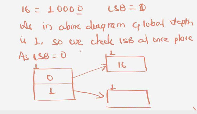
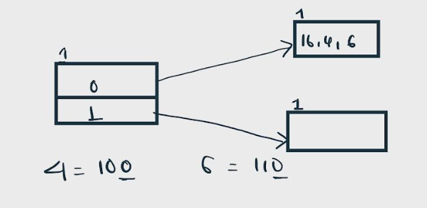
Insert 4 and 6: 

Both 4(100) and 6(110)have 0 in their LSB. Hence, they are also hashed to bucket pointed by Directory 0.

Insert 22: The binary form of 22 is 10110. Its LSB is 0. The bucket pointed by directory 0 is full as the size of the bucket is 3. Hence , there is overflow.

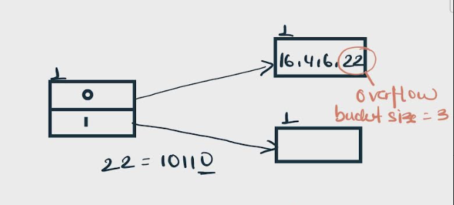
To resolve the overflow , we will split the bucket . 

According to rule 7:

In above case , Local Depth = Global Depth, the bucket splits and directory expansion takes place. 

Also, rehashing of numbers present in the overflowing bucket takes place after the split. And, since the global depth is incremented by 1, now,the global depth is 2. Hence, 16,4,6,22 are now rehashed w.r.t 2 LSBs.[ 16(10000),4(100),6(110),22(10110) ] 

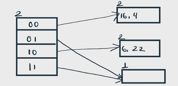
Insert 24 and 10: 24(11000) and 10 (1010) can be hashed based on directories with id 00 and 10. 

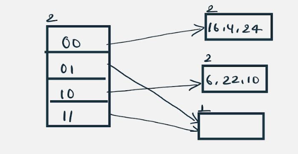
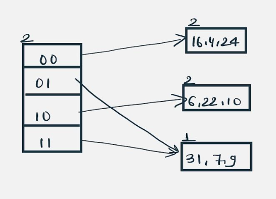
Insert 31,7,9: All of these elements[ 31(11111), 7(111), 9(1001) ] have either 01 or 11 in their LSBs. Hence, they are mapped on the bucket pointed out by 01 and 11. 

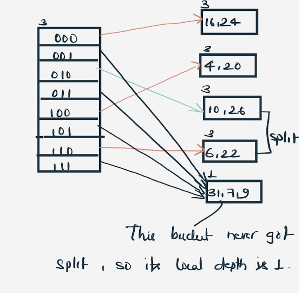
Insert 20: Insertion of data element 20 (10100) will again cause the overflow problem. 

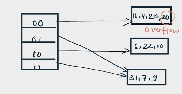
20 is inserted in bucket pointed out by 00. As directed by rule  7-Case 1, since the local depth of the bucket = global-depth, directory expansion (doubling) takes place along with bucket splitting. 

Elements present in overflowing bucket are rehashed with the new global depth. 

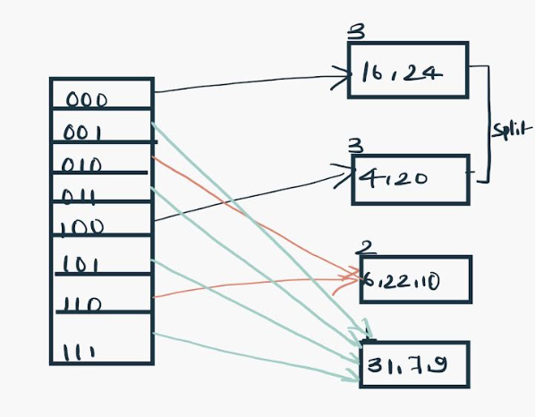
Insert 26: Global depth is 3. Hence, 3 LSBs of 26(11010) are considered. Therefore 26 best fits in the bucket pointed out by directory 010. 

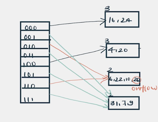
The bucket overflows, and, as directed by rule 7-Case 2, since the local depth of bucket < Global depth (2<3), directories are not doubled but, only the bucket is split and elements are rehashed. 

Finally, the output of hashing the given list of numbers is obtained.