Asymptotic notations: θ , O, Ω , o,ω notations and their properties

Algorithm Efficiency

If a function is linear (without any loops or recursions), the efficiency of that algorithm or the running time of that algorithm can be given as the number of instructions it contains. However, if an algorithm contains loops, then the efficiency of that algorithm may vary depending on the number of loops and the running time of each loop in the algorithm.

Let us consider different cases in which loops determine the efficiency of an algorithm.

Linear Loops

To calculate the efficiency of an algorithm that has a single loop, we need to first determine the number of times the statements in the loop will be executed. This is because the number of iterations is directly proportional to the loop factor. Greater the loop factor, more is the number of iterations. For example, consider the loop given below:

for(i=0;i<100;i++)
  statement block;

Here, 100 is the loop factor. We have already said that efficiency is directly proportional to the number of iterations. Hence, the general formula in the case of linear loops may be given as

f(n) = n

However calculating efficiency is not as simple as is shown in the above example. Consider the loop given below:

for(i=0;i<100;i+=2)

    statement block;

Here, the number of iterations is half the number of the loop factor. So, here the efficiency can be given as

f(n) = n/2

Logarithmic Loops

We have seen that in linear loops, the loop update statement either adds or subtracts the loop-controlling variable. However, in logarithmic loops, the loop-controlling variable is either multiplied or divided during each iteration of the loop. For example, look at the loops given below:

for(i=1;i<1000;i*=2)

   statement block;




for(i=1000;i>=1;i/=2) 

   statement block; 

Consider the first for loop in which the loop-controlling variable i is multiplied by 2. The loop will be executed only 10 times and not 1000 times because in each iteration the value of i doubles. Now, consider the second loop in which the loop-controlling variable i is divided by 2. In this case also, the loop will be executed 10 times. Thus, the number of iterations is a function of the number by which the loop-controlling variable is divided or multiplied. In the examples discussed, it is 2. That is, when n = 1000, the number of iterations can be given by log 1000 which is approximately equal to 10.

Therefore, putting this analysis in general terms, we can conclude that the efficiency of loops in which iterations divide or multiply the loop-controlling variables can be given as

f(n) = log n

Nested Loops

Loops that contain loops are known as nested loops. In order to analyse nested loops, we need to determine the number of iterations each loop completes. The total is then obtained as the product of the number of iterations in the inner loop and the number of iterations in the outer loop.

In this case, we analyse the efficiency of the algorithm based on whether it is a linear logarithmic, quadratic, or dependent quadratic nested loop.

Linear logarithmic loop Consider the following code in which the loop-controlling variable of the inner loop is multiplied after each iteration. The number of iterations in the inner loop is log 10. This inner loop is controlled by an outer loop which iterates 10 times. Therefore, according to the formula, the number of iterations for this code can be given as 10 log 10.

           for(i=0;i<10;i++)

                 for(j=1; j<10;j*=2)

                        statement block;

In more general terms, the efficiency of such loops can be given as f(n) = n log n.

Quadratic loop In a quadratic loop, the number of iterations in the inner loop is equal to the number of iterations in the outer loop. Consider the following code in which the outer loop executes 10 times and for each iteration of the outer loop, the inner loop also executes 10 times. Therefore, the efficiency here is 100.

           for(i=0;i<10;i++)

                 for(j=0; j<10;j++)

                      statement block;

The generalized formula for quadratic loop can be given as f(n) = n^2.

Dependent quadratic loop In a dependent quadratic loop, the number of iterations in the inner loop is dependent on the outer loop. Consider the code given below:

           for(i=0;i<10;i++)

                 for(j=0; j<=i;j++)

                        statement block;

In this code, the inner loop will execute just once in the first iteration, twice in the second iteration, thrice in the third iteration, so on and so forth. In this way, the number of iterations can be calculated as

  1 + 2 + 3 + ... + 9 + 10 = 55

If we calculate the average of this loop (55/10 = 5.5), we will observe that it is equal to the number of iterations in the outer loop (10) plus 1 divided by 2. In general terms, the inner loop iterates (n + 1)/2 times. Therefore, the efficiency of such a code can be given as:

           f(n) = n (n + 1)/2

Asymptotic Analysis

The efficiency of an algorithm depends on the amount of time, storage and other resources required to execute the algorithm. The efficiency is measured with the help of asymptotic notations.An algorithm may not have the same performance for different types of inputs. With the increase in the input size, the performance will change.

The study of change in performance of the algorithm with the change in the order of the input size is defined as asymptotic analysis.

Asymptotic Notations

Asymptotic notations are the mathematical notations used to describe the running time of an algorithm when the input tends towards a particular value or a limiting value.For example: In bubble sort, when the input array is already sorted, the time taken by the algorithm is linear i.e. the best case.

But, when the input array is in reverse condition, the algorithm takes the maximum time (quadratic) to sort the elements i.e. the worst case.

When the input array is neither sorted nor in reverse order, then it takes average time. These durations are denoted using asymptotic notations.There are mainly three asymptotic notations: Theta notation, Omega notation and Big-O notation.

Big-O Notation (O-notation)

Big-O notation represents the upper bound of the running time of an algorithm. Thus, it gives the worst case complexity of an algorithm.

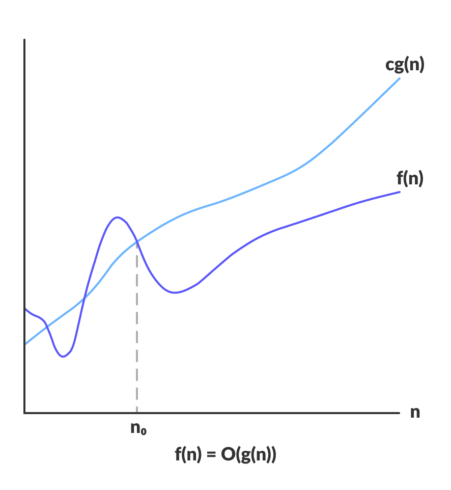
O(g(n)) = { f(n): there exist positive constants c and n0

            such that 0 ≤ f(n) ≤ cg(n) for all n ≥ n0 }

For any value of n, the running time of an algorithm does not cross time provided by O(g(n)).

Since it gives the worst case running time of an algorithm, it is widely used to analyze an algorithm as we are always interested in the worst case scenario.

Omega Notation (Ω-notation)

Omega notation represents the lower bound of the running time of an algorithm. Thus, it provides the best case complexity of an algorithm.

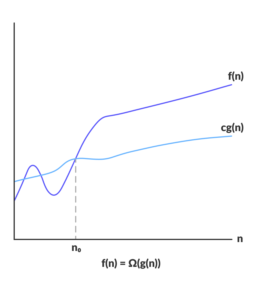
Ω(g(n)) = { f(n): there exist positive constants c and n0 

            such that 0 ≤ cg(n) ≤ f(n) for all n ≥ n0 }

Theta Notation (Θ-notation)

Theta notation encloses the function from above and below. Since it represents the upper and the lower bound of the running time of an algorithm, it is used for analyzing the average case complexity of an algorithm.

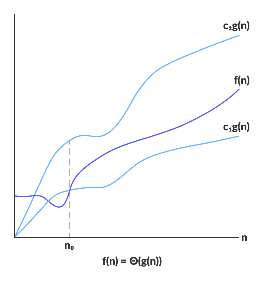
For a function g(n), Θ(g(n)) is given by the relation:

Θ(g(n)) = { f(n): there exist positive constants c1, c2 and n0

            such that 0 ≤ c1g(n) ≤ f(n) ≤ c2g(n) for all n ≥ n0 }

The above expression can be described as a function f(n) belongs to the set Θ(g(n)) if there exist positive constants c1 and c2 such that it can be sandwiched between c1g(n) and c2g(n), for sufficiently large n.

If a function f(n) lies anywhere in between c1g(n) and c2g(n) for all n ≥ n0, then f(n) is said to be asymptotically tight bound.

4. Little O (o):

Definition: Let f(n) and g(n) be two functions defined on the positive integers. We say that f(n) is o(g(n)) (read as "f(n) is little o of g(n)") if for any positive constant c, there exists a constant n₀ such that for all n ≥ n₀, f(n) < c * g(n).

Intuitively, it means that the growth rate of f(n) is strictly less than the growth rate of g(n) for sufficiently large n.Example: If an algorithm's time complexity is o(n²), it means that the running time of the algorithm grows slower than quadratically with the input size.

5. Little Omega (ω):

Definition: Let f(n) and g(n) be two functions defined on the positive integers. We say that f(n) is ω(g(n)) (read as "f(n) is little omega of g(n)") if for any positive constant c, there exists a constant n₀ such that for all n ≥ n₀, f(n) > c * g(n).

Intuitively, it means that the growth rate of f(n) is strictly greater than the growth rate of g(n) for sufficiently large n.Example: If an algorithm's time complexity is ω(n), it means that the running time of the algorithm grows faster than linearly with the input size.

Properties:

1. Reflexivity: For any function f(n), f(n) = θ(f(n)), since any function is asymptotically equivalent to itself.

2. Symmetry: If f(n) = θ(g(n)), then g(n) = θ(f(n)).

3. Transitivity: If f(n) = θ(g(n)) and g(n) = θ(h(n)), then f(n) = θ(h(n)).

4. Multiplicative Constants: If f(n) = θ(g(n)), then kf(n) = θ(kg(n)) for any positive constant k.

5. Additive Constants: If f(n) = θ(g(n)), then f(n) + h(n) = θ(g(n) + h(n)) for any function h(n) such that h(n) = o(g(n)) or h(n) = O(g(n)).